当前位置：首页>学习笔记>大浩浩的笔记课堂——FRM考试学习笔记103

大浩浩的笔记课堂——FRM考试学习笔记103

2026-02-09 20:42:27

Topic 32 Default Probability,Credit Spreads and Credit Derivatives

1.Defaulting probability and recovery rates:

⑴defining default probability:

①survival rate:

A.definition:

It is the probability that a borrower will not default over a specified multi-year period.

B.formulas:

a/ survival rate at end of 2 years:

S₂=(1-d₁)(1-d₂)

b/ survival rate at end of 3 years:

S₃=(1-d₁)(1-d₂)(1-d₃)

·特别注意！

·那么第四年违约的概率为P=(1-d₁)(1-d₂)(1-d₃)d₄

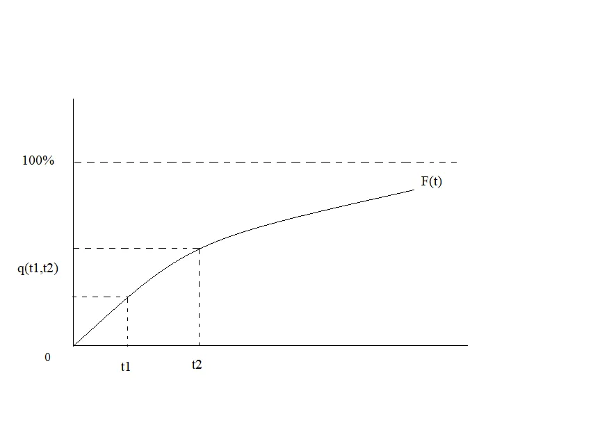
②cumulative default probability(F(t)):

A.definition:

It is the likelihood of counterparty default between the current time period and a future date.

B.characteristic:

It begins at zero and even nearly reaches 100%.

C.formulas:

a/ survival rate at end of 2 years:

C₂=1-S₂=d₁+(1-d₁)d₂

b/ survival rate at end of 3 years:

C₃=1-S₃=d₁+(1-d₁)d₂+(1-d₁)(1-d₂)d₃

③marginal default probability(q(t₁,t₂)):

A.definition:

It is the probability that a borrower will default in any given year.

B.formula:

q(t₁,t₂)=F(t₂)-F(t₁)(t₁≤t₂)

·特别注意！

·So,only the cumulative default probabilities increase over time.

⑵real and risk-neutral default probabilities:

①parameters:

A.real-world parameters:

They are aim to reflect the true value of some financial underlying.

B.risk-neutral parameters:

They reflect parameters derived from market prices.

②probabilities:

A.real default probabilities:

a/ origination:

They are based on historical data.

b/ aim:

They are aimed to reflect the true value of some financial underlying.

c/ representation:

They are the assessment of future default probability for the purpose of risk management or other analysis.

d/ usage:

They are useful for quantitative risk assessment.

B.risk-neutral probabilities:

a/ origination:

It is calculated from market information.

·特别注意！

·credit spread=PD×(1-RR)

b/ representation:

They reflect the market price of default risk and represent estimates of default probability based on observed market prices of securities.

c/ range:

They are materially higher than real-world ones.

d/ usage:

They are useful for hedging consideration.

C.relationships:

risk-neutral default probability

=real default default probability+liquidity premium+default risk premium

So,risk-neutral default probabilities are materially higher than real-world ones.

⑶estimating real default probabilities——historical data:

①Firms with good credit ratings default less often than those with worse ratings.

②different grade credits:

A.investment grade credits:

The default probabilities increase over time:

The increase of cumulative default probability is more than proportional with the horizon.

B.non-investment grade credits:

The default probabilities that increase much less strongly over time(reverse effect):

The increase of cumulative default probability is less than proportional with the horizon,as well as,the cumulative default probability increases much less strongly over time.

C.the reason:

The marginal probability of default increases with maturity for initial high credit ratings,but decreases for initial low credit ratings due to mean reversion effect.

③In computing CVA,not only will the cumulative default probability be important,but also so will the way in which this is distributed marginally.

④Transition practices are more likely to used in the historical approach.

⑷estimating real default probabilities——equity-based approaches:

Defining default probability dynamically:

①Merton-style approach;

②Moody´sKMV:

A.estimation of the market value and volatility of a firm´sassets

B.calculation of the distance to default(standardized measure of default risk)

C.scaling of the distance to default to the actual probability of default using a historical default database

③credit grades.

⑸estimating risk-neutral default probabilities——defined credit spread:

①formulas:

A.the accumulative default probability:

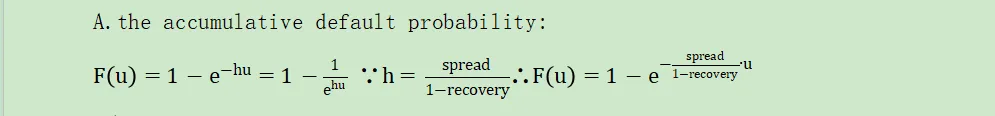
a/ u:a future period

b/ h:the hazard rate of default

·特别注意！

·Hazard rates measure the instantaneous conditional default probability.

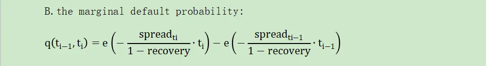
B.the marginal default probability:

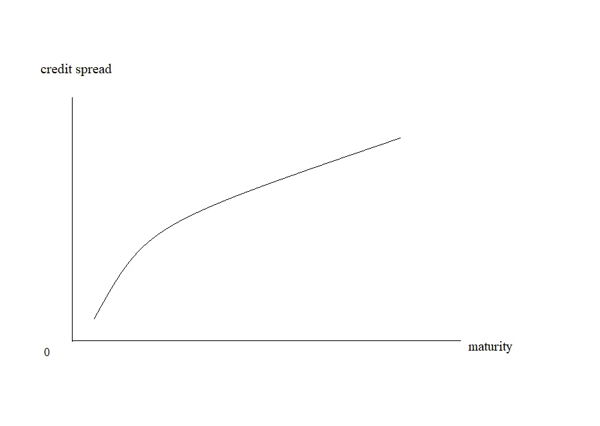
②curves:

The shape of a credit curve plays an important part in determining the distribution of risk-neutral default probability.

A.for an upwards-sloping curve:

Default is less likely in the early years and more likely in the later years.

B.for flat and inverted curve:

Default is reverse.

⑹comparison between real and risk-neutral default probabilities:

①The differences between credit spreads and actual default losses is due to:

A.the relative illiquidity of corporate bonds requiring a liquidity risk premium

B.the limited upside on holding a bond portfolio,or negative skew in bond returns

C.the non diversifiable risk of corporate bonds requiring a systemic risk premium

②the situation to use:

A.not to hedge the default component of counterparty risk

→real world default probabilities

B.intend to hedge against counterparty defaults:

→risk-neutral default probabilities

·特别注意！

·the summary of estimation approaches:

type

characteristic

historical data

approach

1.A transition matrix is helpful in calculating default probabilities because it identifies the historical probabilities of credit rating migration between periods.

2.This methodology assumes the transition matrix is constant over time and hence unaffected by the business cycle,an observation not supported by empirical evidence.In general,credits are more likely to be downgraded than upgraded.

risk-neutral

approach

1.The risk-neutral probability of default is derived from the observed credit spread(to estimate hazard rate used in Poisson process) and the market price of a traded credit security.

2.Empirical evidence indicates that risk-neutral default probabilities are significantly larger than real-world default probabilities.

equity-based

approaches

1.The Merton model:

It uses equity market data to estimate default probabilities.

2.The KMV approach:

It uses a propriety approach built on the Merton model,but it relaxes several

of its assumptions:

⑴Volatility,market value are calculated.

⑵The distance to default is calculated.

⑶Historical default data and distance to default are used.

3.CreditGrades^TM:

⑴using observable date ＆ B/S information

⑵Empirical data is not utilized in this model.

⑺recovery rates:

①loss given default(LGD):

LGD=1-revoery rate

②recovery swap;

③Recoveries tend to be negatively correlated with default rates.

④Recovery rates also depend on the seniority of the claim:

Recovery rates increase with capital structure seniority.

⑤Recovery is related to the timing:

credit event→settled recovery(CDS)→agree OTC derivative claim→final recovery:

A.credit event;

B.settled recovery(CDS):

It could be achieved following the credit event.

C.from settled recovery(CDS) to final recovery:

It is an actual recovery:

a/ Taking long time,may be higher than settled recovery.

b/ Actual recovery is paid on the debt following a bankruptcy or similar process.

·特别注意！

·Recovery rates are lowest during economic downturns,and vary

significantly across industries.

2.Credit default swaps(CDS):

⑴credit derivatives:

They are agreements designed to shift credit risk between parties and their value are derived from the credit performance of corporations,sovereign entities or securities.

·特别注意！

·reference entity 衍生品交易中的参考实体

其是指衍生品交易合约中的一个债券发行方实体。

⑵types of basis:

①single-name basis:

It is a single component such as a corporate.

②portfolio basis:

They are many components such as 125 corporate names.

⑶process of CDS:

①before default:

protection buyer→(premium)→protection seller

②at default:

A.protection buyer→(accrued premium)→protection seller

B.protection buyer←(default settlement)←protection seller

⑷CDS settlement:

①There are fundamentally 2 ways in which this payoff has been achieved in CDSs:

A.physical settlement:

a/ definition:

Deliver the defaulted obligation.

b/ process:

The buyer of the CDS delivers the reference obligation to the seller of

the swap and receives the par value:

△protection buyer→(defaulted securities of the reference entity)→protection seller

△protection buyer←(make a payment of par in cash)←protection seller

c/ advantage:

Delivery squeeze when if the amount of notional required to be delivered is large compared with the amount of outstanding debt.

d/ disadvantage:

There is no need to determine the size of the loss.

B.cash settlement:

a/ definition:

The protection seller will compensate the protection buyer in cash for the value of par minus recovery rate.

·特别注意！

·It requires knowledge of the post-default market price.

b/amount:

(100-Z)%×the notional principal(Z is midpoint)

c/ advantage:

No securities are actually traded(There is no need to own or purchase the defaulted securities),so the risk of delivery squeeze is avoided.

d/ disadvantage:

A problem arises because the market price is fluid and it requires knowledge of the post-default market price.

②The problems of CDS market:

A."naked" CDS position:

A large proportion of protection buyers do not hold the original risk in the form of bonds.

B.delivery squeeze:

If the amount of notional required to be delivered is large compared with amount of outstanding debt.

·特别注意！

·The value of CDS will decrease when the bond price increases.

C.cheapest-to-deliver options:

In physical delivery,they may include low coupons illiquid bonds.

·特别注意！

·The problems of delivery squeeze and cheapest-to-deliver options have been limited by the adoption of an auction protocol in setting credit events.

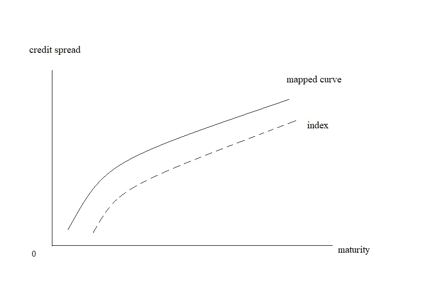
3.Curve mapping:

⑴basic of mapping:

⑵curve shape:

4.Portfolio credit derivatives:

⑴CDS index:

①products(most popular):

A.DJ CDX NAIG:

125 North American investment-grade reference entities(equally weighted)

B.DJ iTraxx Europe:

125 European corporate investment-grade reference entities(equally weighted)

②definition:

CDS indices are created with a fixed maturity and static constituents.If there is a significant credit event,the affected credit entity will be removed,but not replaced,

from the index.

③features:

They "roll" every 6 months.

A.A roll will involve:

a/ adjustment of maturity:

5,7 and 10 years

b/ adjustment of portfolio:

To replace defaulted names and maintain a homogenous credit quality.

c/ premium:

fixed—100 or 500 bps.

B.Rolls only influence new trades and not existing ones.

⑵index tranches:

①including:

super senior→senior→mezzanine→equity:

②characteristic:

Each tranche is described by its attachment point(X%) and detachment point(Y%),denoted [X%,Y%],and the width of each tranche is (Y%-X%).

⑶super senior risk:

①super senior tranches:

A.They represent the portion of the capital structure for credit indices that has the highest subordination level and lowest probability of incurring losses because their attachment points are much higher in the capital structure.

B.Informally,these tranches are termed super triple-A and quadruple-A tranches.

②the formula:

A.X:the attachment point of the tranche(%)

B.n:the number of names in the index

C.recovery:the average recovery rate for the defaults that occur

③the risk:

A.The primary risk of these ranches is counterparty risk(termed

super-senior risk) as this risk is positively correlated to tranche seniority.That is,higher seniority tranches have higher levels of counterparty risk.

B.It is nearly impossible for institutions to efficiently hedge this super-senior risk.

⑷collateralized debt obligation(CDO):

CDOs can be broadly divided into 2 categories:

①synthetic CDOs or collateralized synthetic obligations(CSOs):

They are similar to index tranches.

②structured finance securities:

A.It covers cash CDOs,collateralized loan obligations(CLOs),MBS,and CDOs of ABSs.

B.the differences with synthetic CDOs:

The structure and tranche losses occur by means of a much more complex mechanism.

大浩浩的笔记课堂之FRM考试学习笔记合集