📖 源码:https://github.com/mambo-wang/ai-agent
Phase 2: NLP 核心技术与 Transformer 基础
学习周期:2026-04-06 至 2026-04-11
本笔记涵盖:向量数据库、Self-Attention、位置编码、完整 Transformer 架构
目录
- Day 7: 向量数据库与 Embedding
- Day 8: Self-Attention 自注意力机制
- Day 9: Positional Encoding 位置编码
- Day 10: Transformer 完整架构
- 核心概念总结
Day 7: 向量数据库与 Embedding
7.1 什么是 Embedding?
Embedding(嵌入) 是将离散的非结构化数据(文字、图片、音频等)转换为连续的稠密向量的技术。
~/ai-agent
文字 → 嵌入向量
"苹果"  → [0.23, -0.45, 0.87, ...] (假设 384 维)
"水果"  → [0.18, -0.52, 0.91, ...]
"汽车"  → [-0.33, 0.78, -0.12, ...]
核心特性:
- 语义相似 → 向量相近:在向量空间中,"苹果"和"水果"的距离比"苹果"和"汽车"更近
- 维度固定:通常 128/256/384/768/1024/1536 维等
- 可计算:向量加减、点积、余弦相似度
7.2 相似度计算
向量间的相似度通常用以下方式衡量:
余弦相似度 (Cosine Similarity):
~/ai-agent
cosine(A, B) = (A · B) / (||A|| × ||B||)
值范围 [-1, 1],越接近 1 表示越相似。
欧氏距离 (Euclidean Distance):
~/ai-agent
dist(A, B) = ||A - B||
距离越小表示越相似。
7.3 预训练 Embedding 模型
常用模型:sentence-transformers 库提供开箱即用的文本嵌入模型:
| 模型名称 |
向量维度 |
特点 |
all-MiniLM-L6-v2 |
384 |
速度快,效果好 |
all-mpnet-base-v2 |
768 |
效果更好,速度较慢 |
BAAI/bge-large-zh-v1.5 |
1024 |
中文优化 |
7.4 什么是向量数据库?
向量数据库是专门用于存储和检索高维向量的数据库系统。
为什么需要向量数据库?
- 普通数据库无法高效处理向量相似度搜索
- 当数据量达到百万级时,暴力搜索(逐个计算距离)太慢
- 向量数据库使用近似最近邻 (ANN) 算法加速检索
7.5 主流向量数据库对比
| 数据库 |
特点 |
适用场景 |
| Milvus |
开源、功能强大、云原生 |
大规模生产环境 |
| Pinecone |
云服务、免运维 |
快速上手 |
| Chroma |
轻量级、本地优先 |
个人项目、小规模 |
| FAISS |
Facebook 开源、GPU 加速 |
研究、离线场景 |
| Qdrant |
Rust 实现、高性能 |
需要高性能的场景 |
7.6 Demo 代码:Milvus 向量数据库实战
~/ai-agent
# day7_vector_db.py - 向量数据库示例:文本相似性搜索
# 依赖: pip install sentence-transformers pymilvus

from sentence_transformers import SentenceTransformer  # 文本向量化库
from pymilvus import MilvusClient                      # Milvus 客户端

# ============ 1. 初始化 ============
# 加载预训练模型:all-MiniLM-L6-v2,输出 384 维向量
model = SentenceTransformer("all-MiniLM-L6-v2")

# 连接到本地 Milvus 数据库文件(如果不存在会自动创建)
client = MilvusClient(uri="./milvus_demo.db")

# ============ 2. 准备文档 ============
docs = [
    "我喜欢吃苹果",     # 与苹果相关
    "今天天气很好",     # 天气相关
    "苹果是一种水果",   # 水果定义
    "明天可能会下雨",   # 天气预测
    "香蕉也是水果"      # 水果定义
]

# ============ 3. 生成向量 ============
# encode: 将每个句子转换为 384 维向量
vectors = model.encode(docs).tolist()

# ============ 4. 存入 Milvus ============
client.create_collection(
    collection_name="my_docs",
    dimension=384,              # 向量维度,必须与模型输出一致
    overwrite=True              # 覆盖已存在的集合
)

client.insert(
    collection_name="my_docs",
    data=[
        {"id": i, "text": docs[i], "vector": vectors[i]}
        for i in range(len(docs))
    ]
)

# ============ 5. 查询 ============
query = "水果"  # 查询关键词
query_vector = model.encode([query]).tolist()[0]

results = client.search(
    collection_name="my_docs",
    data=[query_vector],
    limit=3,                    # 返回最相似的 3 个结果
    output_fields=["text"]
)

# ============ 6. 打印结果 ============
print(f"查询: {query}")
print("=" * 40)
for i, result in enumerate(results[0]):
    print(f"Top {i+1}: {result['entity']['text']} (距离: {result['distance']:.4f})")

# ============ 输出示例 ============
# 查询: 水果
# ========================================
# Top 1: 苹果是一种水果 (距离: 0.8942)
# Top 2: 香蕉也是水果 (距离: 0.8721)
# Top 3: 我喜欢吃苹果 (距离: 0.6234)
7.7 RAG 架构中的向量数据库
向量数据库是 RAG (Retrieval-Augmented Generation) 系统的核心组件:
~/ai-agent
RAG 工作流程:
1. 索引阶段:将文档切成块,每块生成向量,存入向量数据库
2. 检索阶段:用户问题转为向量,检索最相关的文档块
3. 生成阶段:将检索到的文档和问题一起发给 LLM 生成回答
7.8 Day 7 小结
| 概念 |
理解要点 |
| Embedding |
文字 → 固定维度向量,语义相近的词向量也相近 |
| 相似度 |
余弦相似度、欧氏距离 |
| 向量数据库 |
存储和检索高维向量,支持 ANN 加速 |
| RAG |
检索增强生成,向量数据库是核心组件 |
Day 8: Self-Attention 自注意力机制
8.1 为什么需要注意力机制?
在处理序列数据时,传统的 RNN/LSTM 存在以下问题:
- 长距离依赖困难:信息需要经过很多时间步才能传递,容易梯度消失
- 无法并行:必须顺序处理,计算效率低
- 难以捕捉远距离关系:"The animal didn't cross the street because it was too tired" — "it" 指代 "animal",但 RNN 可能早就忘了
8.2 Self-Attention 的核心思想
Self-Attention(自注意力) 的核心是:序列中每个位置都"看"所有其他位置,计算它们之间的相关性。
~/ai-agent
输入序列: ["The", "cat", "sat", "on", "the", "mat"]

"The"  看所有词 → 发现自己和 "cat" 关系不大
"cat"  看所有词 → 发现 "sat" 是自己的动作,关联最强
"it"   看所有词 → 发现 "cat" 是自己的前指,关联最强
8.3 Q, K, V 三个向量
Self-Attention 使用三个向量:
| 向量 |
含义 |
作用 |
| Q (Query) |
查询 |
"我想要查找什么信息" |
| K (Key) |
键 |
"我包含什么信息,可以被查询匹配" |
| V (Value) |
值 |
"信息的实际内容" |
类比:
- Q 就像搜索引擎中的搜索词
- K 就像每个网页的标题/关键词
- V 就像网页的实际内容
- 搜索引擎用 Q 和 K 匹配程度来决定返回哪些 V
8.4 Attention 计算公式
~/ai-agent
Attention(Q, K, V) = softmax(QK^T / √d_k) × V
计算步骤:
~/ai-agent
Step 1: QKV 变换
  Q = X × W_Q
  K = X × W_K
  V = X × W_V

Step 2: 计算注意力分数
  scores = Q × K^T / √d_k

Step 3: Softmax 归一化
  weights = softmax(scores)

Step 4: 加权求和
  output = weights × V
为什么要除以 √d_k?
- d_k 越大,点积的值越大
- 过大的值导致 softmax 梯度接近 0
- 除以 √d_k 保持方差稳定
8.5 Multi-Head Attention(多头注意力)
单个注意力头可能只学到一个方面的关系。多头注意力让模型同时学习多种关系:
~/ai-agent
头1:学习主谓关系 (The cat → sat)
头2:学习定语关系 (the → mat)
头3:学习指代关系 (it → cat)
头4:学习邻近关系 (on → the)
...
最后把所有头的输出拼接起来,再做一次线性变换。
8.6 Demo 代码:Self-Attention 实现
~/ai-agent
# day08_self_attention.py - Self-Attention 可视化

import torch
import torch.nn.functional as F
import matplotlib.pyplot as plt
import seaborn as sns
import math

class SelfAttention:
    """
    简化的 Self-Attention 实现

    核心概念:
    - Q (Query): 查询向量,"我想要查找什么信息"
    - K (Key): 键向量,"我包含什么信息"
    - V (Value): 值向量,"信息的实际内容"
    """

    def __init__(self, d_model: int, num_heads: int = 1):
        self.d_model = d_model
        self.num_heads = num_heads
        self.d_k = d_model // num_heads

        # 初始化 Q, K, V 的投影矩阵
        torch.manual_seed(42)
        self.W_Q = torch.randn(d_model, d_model) * 0.1
        self.W_K = torch.randn(d_model, d_model) * 0.1
        self.W_V = torch.randn(d_model, d_model) * 0.1

    def forward(self, x: torch.Tensor, mask: torch.Tensor = None):
        """
        前向传播:计算 Self-Attention

        参数:
            x: 输入序列 [seq_len, d_model]
            mask: 掩码张量(可选)

        返回:
            output: 注意力加权后的输出 [seq_len, d_model]
            attention_weights: 注意力权重矩阵 [seq_len, seq_len]
        """
        seq_len = x.shape[0]

        # ========== Step 1: 计算 Q, K, V ==========
        Q = torch.matmul(x, self.W_Q)  # [seq_len, d_model]
        K = torch.matmul(x, self.W_K)
        V = torch.matmul(x, self.W_V)

        # ========== Step 2: 计算 Attention Score ==========
        # scores[i][j] = Query[i] 对 Key[j] 的相关性
        scores = torch.matmul(Q, K.transpose(-2, -1))  # [seq_len, seq_len]

        # 缩放:防止 d_k 过大导致梯度消失
        scores = scores / math.sqrt(self.d_k)

        # ========== Step 3: 应用 Mask(可选)============
        if mask is not None:
            scores = scores.masked_fill(mask == 0, float('-inf'))

        # ========== Step 4: Softmax 得到注意力权重 ==========
        attention_weights = F.softmax(scores, dim=-1)

        # ========== Step 5: 加权求和 ==========
        output = torch.matmul(attention_weights, V)

        return output, attention_weights


def tokenize(text: str):
    """简单分词"""
    return text.lower().split()


def create_embeddings(tokens: list, d_model: int):
    """创建词嵌入向量"""
    torch.manual_seed(42)
    return torch.randn(len(tokens), d_model) * 0.1


def visualize_attention(tokens, attention_weights, title="Self-Attention Heatmap"):
    """绘制注意力热力图"""
    weights = attention_weights.detach().numpy()

    fig, ax = plt.subplots(figsize=(10, 8))
    sns.heatmap(
        weights,
        annot=True,
        fmt='.2f',
        cmap='Blues',
        xticklabels=tokens,
        yticklabels=tokens,
        ax=ax,
        vmin=0,
        vmax=1
    )
    ax.set_xlabel('Key (被注意的词)')
    ax.set_ylabel('Query (主动注意的词)')
    ax.set_title(title)

    plt.tight_layout()
    plt.savefig('attention_heatmap.png', dpi=150)
    print(f"✅ 热力图已保存: attention_heatmap.png")


def main():
    TEXT = "The cat sat on the mat because it was tired"
    D_MODEL = 64
    NUM_HEADS = 1

    print("=" * 50)
    print("Day 8 Demo: Self-Attention 可视化")
    print("=" * 50)

    # 分词
    tokens = tokenize(TEXT)
    print(f"\n📝 输入: \"{TEXT}\"")
    print(f"📦 Token: {tokens}")

    # 创建词嵌入
    embeddings = create_embeddings(tokens, D_MODEL)
    print(f"📐 向量维度: {embeddings.shape}")

    # 计算 Self-Attention
    attention = SelfAttention(d_model=D_MODEL, num_heads=NUM_HEADS)
    output, attn_weights = attention.forward(embeddings)

    print(f"\n🧠 注意力权重矩阵形状: {attn_weights.shape}")

    # 打印注意力权重
    print("\n🔍 Attention 权重矩阵 (行=Query, 列=Key):")
    header = "        " + "  ".join([f"{t[:4]:>4}" for t in tokens])
    print(header)
    for i, token in enumerate(tokens):
        row = attn_weights[i]
        row_str = "  ".join([f"{v:.2f}" for v in row])
        print(f"{token[:4]:>4}  {row_str}")

    # 分析每个词最关注什么
    print("\n💡 每个词最关注的 token:")
    for i, token in enumerate(tokens):
        row = attn_weights[i].clone()
        row[i] = -1  # 排除自己
        max_idx = row.argmax().item()
        max_weight = attn_weights[i, max_idx].item()
        print(f"  '{token}' → '{tokens[max_idx]}' (权重: {max_weight:.3f})")

    # 生成热力图
    visualize_attention(tokens, attn_weights, f"Self-Attention: \"{TEXT}\"")


if __name__ == "__main__":
    main()
8.7 Attention 可视化解读
运行后会生成热力图:
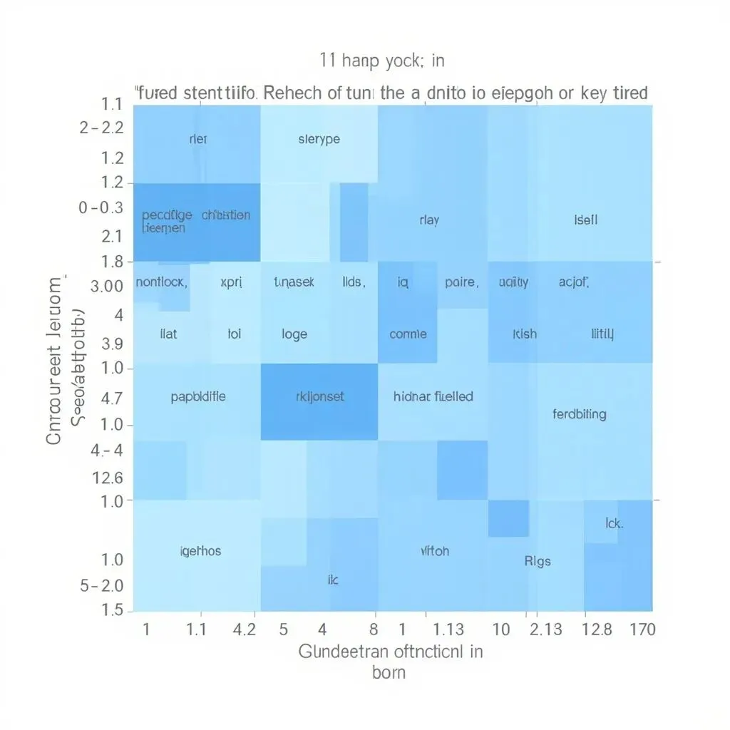
8.8 Day 8 小结
| 概念 |
理解要点 |
| Self-Attention |
每个位置看所有位置,建立全局依赖 |
| Q, K, V |
Query=查询,Key=匹配条件,Value=实际内容 |
| Attention Score |
QK^T / √d_k,体现相关性 |
| Softmax |
将分数归一化为概率分布(权重) |
| Multi-Head |
多头并行学习不同类型的关联 |
Day 9: Positional Encoding 位置编码
9.1 为什么需要位置编码?
Self-Attention 本身不包含位置信息!
看这个例子:
~/ai-agent
"A 打了 B" → "A hit B"
"B 打了 A" → "B hit A"

Self-Attention 的计算完全一样!
因为它只关心"相关性",不关心"谁在谁前面"
这意味着:
- "A 打了 B" 和 "B 打了 A" 在 Attention 看来是一样的
- 词序信息完全丢失了!
9.2 位置编码的解决方案
解决方案:给每个位置一个独特的"位置向量",加到词嵌入上。
~/ai-agent
词 "爱" 在位置 0:  embed("爱") + position_encoding(0)
词 "我" 在位置 1:  embed("我") + position_encoding(1)
词 "中" 在位置 2:  embed("中") + position_encoding(2)
9.3 Sinusoidal 位置编码
Google 在原始 Transformer 论文中提出了 Sinusoidal 编码:
~/ai-agent
PE(pos, 2i)   = sin(pos / 10000^(2i/d_model))
PE(pos, 2i+1) = cos(pos / 10000^(2i/d_model))

其中:
- pos: 位置 (0, 1, 2, ...)
- i: 维度索引 (0, 1, 2, ..., d_model/2)
- d_model: 词向量维度
直观理解:
- 低维度 i:小数字做分母 → 高频波形 → 变化快 → 关注精细位置
- 高维度 i:大数字做分母 → 低频波形 → 变化慢 → 关注粗粒度位置
9.4 为什么选择 Sinusoidal?
| 特性 |
说明 |
| 可外推 |
可以计算任意位置的编码,不限于训练长度 |
| 唯一性 |
每个位置有唯一的编码 |
| 相对位置 |
sin(A-B) 和 cos(A-B) 可由 sin(A), cos(A), sin(B), cos(B) 线性组合得到 |
| 平滑性 |
相邻位置的编码相似 |
9.5 其他位置编码方式
| 编码方式 |
说明 |
代表模型 |
| Sinusoidal |
固定公式,无需学习 |
原版 Transformer |
| Learned Absolute |
可学习的绝对位置 |
BERT |
| RoPE |
旋转编码,相对位置 |
Llama, GLM |
| ALiBi |
线性偏置 |
BLOOM |
9.6 RoPE(旋转位置编码)简介
RoPE 是目前最流行的相对位置编码之一,被 Llama 等模型采用。
核心思想:不是把位置编码加到词向量上,而是旋转词向量。
~/ai-agent
旋转矩阵 R(m) = [[cos(mθ), -sin(mθ)],
                [sin(mθ),  cos(mθ)]]
优点:
- 理论上有更好的外推能力
- 计算高效
9.7 Demo 代码:位置编码实现
~/ai-agent
# day09_positional_encoding.py - 位置编码详解

import torch
import numpy as np
import matplotlib.pyplot as plt
import seaborn as sns
import math

class PositionalEncoding:
    """
    Sinusoidal 位置编码实现

    公式:
    PE(pos, 2i)   = sin(pos / 10000^(2i/d))
    PE(pos, 2i+1) = cos(pos / 10000^(2i/d))

    特点:
    1. 每个位置有唯一编码
    2. 可以泛化到任意长度
    3. 允许模型学习相对位置
    """

    def __init__(self, d_model: int, max_len: int = 5000, dropout: float = 0.1):
        self.d_model = d_model
        self.max_len = max_len
        self.dropout = torch.nn.Dropout(p=dropout)

        # 预计算位置编码表
        pe = self._create_encoding_table(max_len, d_model)
        self.pe = pe

    def _create_encoding_table(self, max_len: int, d_model: int) -> torch.Tensor:
        """创建位置编码表"""
        pe = torch.zeros(max_len, d_model)

        # 位置索引
        position = torch.arange(0, max_len, dtype=torch.float).unsqueeze(1)  # [max_len, 1]

        # 频率指数
        div_term = torch.exp(
            torch.arange(0, d_model, 2, dtype=torch.float) *
            (-math.log(10000.0) / d_model)
        )
        # div_term[i] = 10000^(-2i/d_model)

        # 偶数维度:sin
        pe[:, 0::2] = torch.sin(position * div_term)
        # 奇数维度:cos
        pe[:, 1::2] = torch.cos(position * div_term)

        # 添加 batch 维度
        pe = pe.unsqueeze(0)  # [1, max_len, d_model]

        return pe

    def forward(self, x: torch.Tensor) -> torch.Tensor:
        """
        将位置编码添加到输入

        参数:
            x: [batch_size, seq_len, d_model] 或 [seq_len, d_model]
        """
        if x.dim() == 3:
            seq_len = x.size(1)
        else:
            seq_len = x.size(0)

        # 取出对应长度的位置编码
        position_encoding = self.pe[:, :seq_len, :].to(x.device)

        # 残差连接
        x = x + position_encoding

        return self.dropout(x)


def demonstrate_position_encoding():
    """演示位置编码的数学特性"""
    d_model = 64
    max_len = 100

    pe = PositionalEncoding(d_model=d_model, max_len=max_len)
    encoding_table = pe.pe[0].numpy()

    print("=" * 60)
    print("Positional Encoding 数学特性演示")
    print("=" * 60)

    # 不同位置的编码差异
    print("\n📍 位置 0 vs 位置 1 的编码(前 8 维):")
    print(f"  位置 0: {encoding_table[0, :8].round(3)}")
    print(f"  位置 1: {encoding_table[1, :8].round(3)}")

    # 计算余弦相似度
    from sklearn.metrics.pairwise import cosine_similarity

    sample_indices = [0, 1, 2, 3, 4, 9, 19, 49, 99]
    samples = encoding_table[sample_indices]
    similarities = cosine_similarity(samples)

    print("\n🔗 位置之间的余弦相似度:")
    print(f"  位置: {sample_indices}")
    for i, idx in enumerate(sample_indices):
        row = [f"{sim:.2f}" for sim in similarities[i]]
        print(f"  位置 {idx:2d}: {row}")

    print("\n📈 相邻位置 vs 远距离位置的相似度:")
    print(f"  位置 0 vs 1 (距离=1): {similarities[0, 1]:.4f}")
    print(f"  位置 0 vs 10 (距离=10): {similarities[0, 6]:.4f}")
    print(f"  位置 0 vs 100 (距离=100): {similarities[0, 8]:.4f}")

    return encoding_table


def visualize_position_encoding(encoding_table: np.ndarray):
    """可视化位置编码"""
    max_len, d_model = encoding_table.shape

    # ========== 图1: 热力图 ==========
    fig1, ax1 = plt.subplots(figsize=(14, 8))
    sns.heatmap(
        encoding_table.T,
        cmap='RdBu_r',
        center=0,
        ax=ax1,
        cbar_kws={'label': 'Encoding Value'}
    )
    ax1.set_xlabel('Position (位置)')
    ax1.set_ylabel('Dimension (维度)')
    ax1.set_title('Positional Encoding Heatmap')

    plt.tight_layout()
    plt.savefig('position_encoding_heatmap.png', dpi=150)
    print("✅ 热力图已保存: position_encoding_heatmap.png")

    # ========== 图2: 不同维度的波形 ==========
    fig2, axes = plt.subplots(2, 2, figsize=(14, 8))
    dimensions = [0, 1, 2, 32]
    positions = np.arange(max_len)

    for ax, dim in zip(axes.flat, dimensions):
        values = encoding_table[:, dim]
        wave_type = 'sin' if dim % 2 == 0 else 'cos'
        color = 'blue' if dim % 2 == 0 else 'red'

        ax.plot(positions, values, color=color, linewidth=1.5)
        ax.set_title(f'维度 {dim} ({wave_type})')
        ax.set_xlabel('Position')
        ax.set_ylabel('Value')
        ax.grid(True, alpha=0.3)
        ax.set_ylim([-1.1, 1.1])

    plt.suptitle('不同维度的正弦/余弦波形\n低维度变化快,高维度变化慢')
    plt.tight_layout()
    plt.savefig('position_encoding_waves.png', dpi=150)
    print("✅ 波形图已保存: position_encoding_waves.png")


def visualize_batch_effect():
    """演示位置编码的作用"""
    print("\n" + "=" * 60)
    print("💡 位置编码的作用演示")
    print("=" * 60)

    torch.manual_seed(42)
    word_embeddings = torch.randn(4, 8) * 0.1

    pe = PositionalEncoding(d_model=8, max_len=10)

    # 模拟句子 "I think you are good" -> 词索引 [0, 1, 2, 3]
    sentence_indices = [0, 1, 2, 3]

    print("\n📝 原始词嵌入:")
    print(f"  词 0: {word_embeddings[0].numpy().round(3)}")
    print(f"  词 1: {word_embeddings[1].numpy().round(3)}")

    # 添加位置编码
    enhanced_embeddings = []
    for i, word_idx in enumerate(sentence_indices):
        enhanced = word_embeddings[word_idx] + pe.pe[0, i]
        enhanced_embeddings.append(enhanced)

    enhanced_embeddings = torch.stack(enhanced_embeddings)

    print("\n✨ 添加位置编码后:")
    print(f"  位置0: {enhanced_embeddings[0].numpy().round(3)[:5]}...")
    print(f"  位置1: {enhanced_embeddings[1].numpy().round(3)[:5]}...")

    from sklearn.metrics.pairwise import cosine_similarity

    word_sim = cosine_similarity(word_embeddings[sentence_indices])
    enhanced_sim = cosine_similarity(enhanced_embeddings.detach().numpy())

    print("\n🔍 相似度对比:")
    print(f"  原始词嵌入 词0 vs 词1 相似度: {word_sim[0, 1]:.4f}")
    print(f"  添加位置编码后 位置0 vs 位置1 相似度: {enhanced_sim[0, 1]:.4f}")

    print("\n🎯 关键点:同一词在不同位置变得可区分!")


def main():
    print("=" * 60)
    print("Day 9 Demo: Positional Encoding(位置编码)")
    print("=" * 60)

    # 数学特性演示
    encoding_table = demonstrate_position_encoding()

    # 可视化
    print("\n🎨 生成可视化图表...")
    visualize_position_encoding(encoding_table)

    # 位置编码作用演示
    visualize_batch_effect()

    print("\n" + "=" * 60)
    print("✅ Day 9 学习完成!")
    print("=" * 60)


if __name__ == "__main__":
    main()
9.8 位置编码可视化解读
生成了位置编码可视化图:
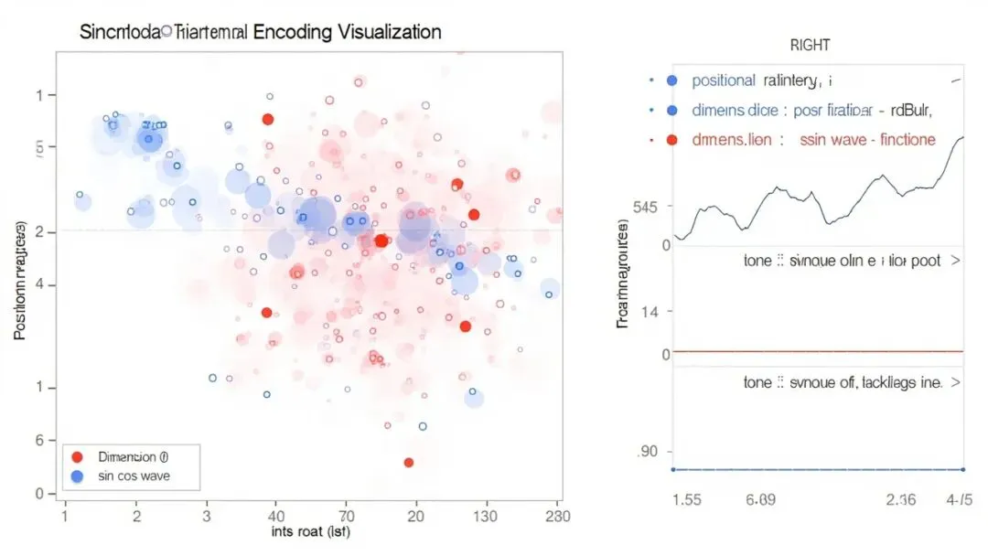
2. position_encoding_waves.png — 波形图
~/ai-agent
维度 0 (sin):  ~~~高频~~~  变化最快
维度 1 (cos):  ~~~高频~~~
维度 2 (sin):  ~~中频~~   变化中等
维度 32 (cos):  -低频-    变化最慢
9.9 Day 9 小结
| 概念 |
理解要点 |
| 位置编码的必要性 |
Self-Attention 不含位置信息,需要注入 |
| Sinusoidal 编码 |
不同频率的 sin/cos 函数组合 |
| 可外推 |
可以计算任意长度,不限于训练长度 |
| 相对位置 |
sin(A-B) 可以表示相对位置关系 |
| RoPE |
旋转编码,更好的外推能力 |
Day 10: Transformer 完整架构
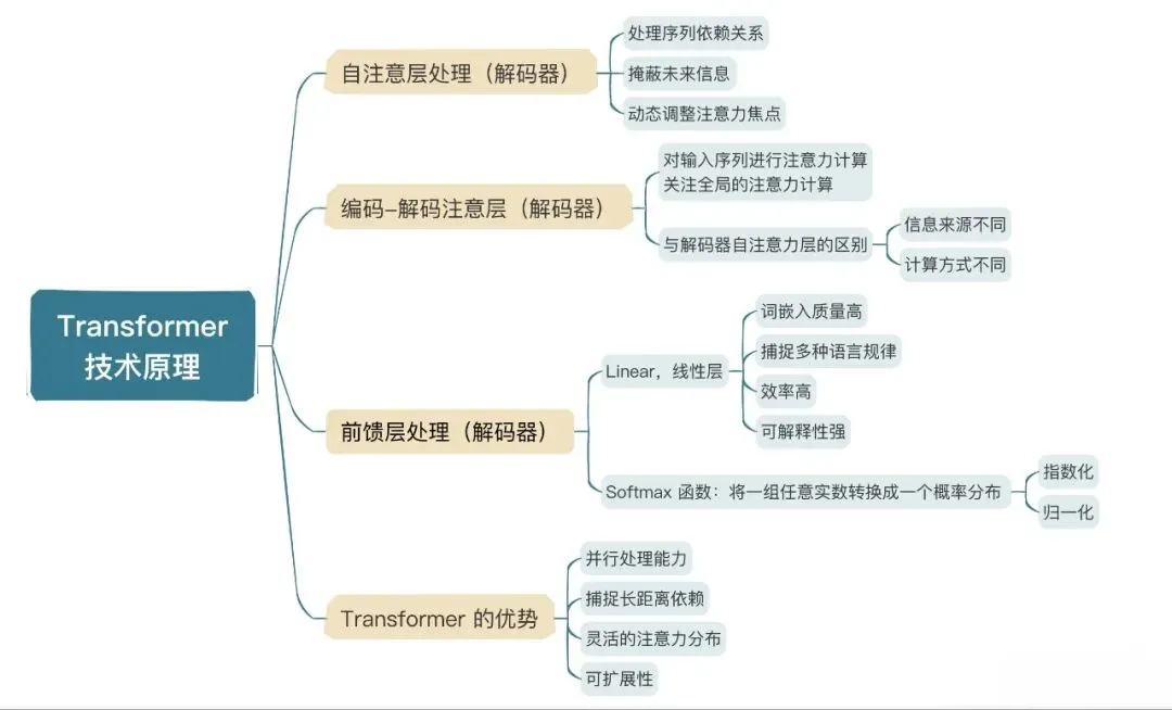
10.1 Transformer 整体架构
Transformer 由 Encoder(编码器) 和 Decoder(解码器) 两部分组成:
~/ai-agent
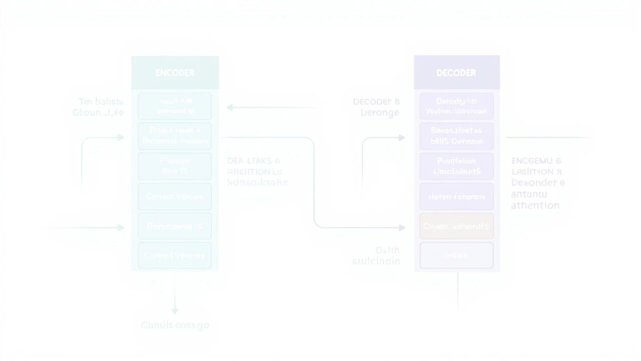
10.2 Encoder 详解
每个 Encoder 层包含两个子层:
① Multi-Head Self-Attention
- 每个位置"看"序列中所有位置
- 建立词与词之间的关联
② Position-wise Feed-Forward Network
~/ai-agent
FFN(x) = max(0, xW₁ + b₁)W₂ + b₂
- 两层线性变换,中间有 ReLU 激活
- 对每个位置独立进行非线性变换
③ 残差连接 + Layer Normalization
~/ai-agent
output = LayerNorm(x + Sublayer(x))
- 残差连接:让梯度直接回传
- Layer Norm:稳定训练
10.3 Decoder 详解
每个 Decoder 层包含三个子层:
① Masked Self-Attention(遮蔽自注意力)
- 确保生成时不能看到"未来"的词
- 训练时使用 Teacher Forcing
② Cross Attention(交叉注意力)
- Q 来自 Decoder
- K, V 来自 Encoder 输出
- 作用:让 Decoder 能"看" Encoder 的信息
③ Feed-Forward Network
- 同 Encoder
10.4 Mask 的作用
因果 Mask(Causal Mask):
~/ai-agent
序列: "<SOS> 我 爱 机器 学习"

位置0 "我": 只能看 "我"
位置1 "爱": 只能看 "我 爱"
位置2 "机": 只能看 "我 爱 机"
位置3 "器": 只能看 "我 爱 机器"
位置4 "学": 只能看 "我 爱 机器 学"
Padding Mask:
- 忽略 padding 的位置
10.5 Layer Normalization vs Batch Normalization
| 特性 |
Layer Norm |
Batch Norm |
| 归一化维度 |
单个样本内 |
跨 batch |
| NLP 适用性 |
✅ 适合 |
❌ 不适合 |
| 序列长度变化 |
✅ 稳定 |
❌ 不稳定 |
10.6 完整 Demo 代码
~/ai-agent
# day10_transformer.py - Transformer 完整架构(纯 NumPy 版)
import numpy as np
import matplotlib
matplotlib.use('Agg')
import matplotlib.pyplot as plt
import math
# ===================== Softmax 和 Mask =====================
def softmax(x, axis=-1):
"""Softmax 函数"""
exp_x = np.exp(x - np.max(x, axis=axis, keepdims=True))
return exp_x / np.sum(exp_x, axis=axis, keepdims=True)
def create_causal_mask(seq_len):
"""
创建下三角 mask(因果 mask)
作用:Decoder 生成时,不能看到 "未来" 的词
"""
mask = np.triu(np.ones((seq_len, seq_len)), k=1)
return np.where(mask == 1, float('-inf'), 0.0)
# ===================== 位置编码 =====================
class PositionalEncoding:
"""Sinusoidal 位置编码"""
def __init__(self, d_model, max_len=5000):
self.d_model = d_model
self.pe = self._create_encoding(max_len)
def _create_encoding(self, max_len):
pe = np.zeros((max_len, self.d_model))
position = np.arange(max_len).reshape(-1, 1)
div_term = np.exp(
np.arange(0, self.d_model, 2) * (-math.log(10000.0) / self.d_model)
)
pe[:, 0::2] = np.sin(position * div_term)
pe[:, 1::2] = np.cos(position * div_term)
return pe
def add(self, x):
seq_len = x.shape[1]
return x + self.pe[:seq_len]
# ===================== Scaled Dot-Product Attention =====================
def scaled_dot_product_attention(Q, K, V, mask=None):
"""
Scaled Dot-Product Attention
公式: Attention(Q,K,V) = softmax(QK^T / √d_k) × V
"""
d_k = Q.shape[-1]
# 1. 计算点积
scores = np.matmul(Q, K.T)
# 2. 缩放
scores = scores / math.sqrt(d_k)
# 3. 应用 mask
if mask is not None:
scores = scores + mask
# 4. Softmax
attention_weights = softmax(scores, axis=-1)
# 5. 加权求和
output = np.matmul(attention_weights, V)
return output, attention_weights
# ===================== Multi-Head Attention =====================
class MultiHeadAttention:
"""多头注意力"""
def __init__(self, d_model, n_heads):
assert d_model % n_heads == 0
self.d_model = d_model
self.n_heads = n_heads
self.d_k = d_model // n_heads
np.random.seed(42)
self.W_Q = np.random.randn(d_model, d_model) * 0.02
self.W_K = np.random.randn(d_model, d_model) * 0.02
self.W_V = np.random.randn(d_model, d_model) * 0.02
self.W_O = np.random.randn(d_model, d_model) * 0.02
def forward(self, Q, K, V, mask=None):
batch = Q.shape[0]
seq_len = Q.shape[1]
# 1. QKV 线性变换
Q = np.matmul(Q, self.W_Q)
K = np.matmul(K, self.W_K)
V = np.matmul(V, self.W_V)
# 2. 分成多个头
Q = Q.reshape(batch, seq_len, self.n_heads, self.d_k).transpose(0, 2, 1, 3)
K = K.reshape(batch, -1, self.n_heads, self.d_k).transpose(0, 2, 1, 3)
V = V.reshape(batch, -1, self.n_heads, self.d_k).transpose(0, 2, 1, 3)
# 3. 计算 Attention
scores = np.matmul(Q, K.transpose(0, 1, 3, 2)) / math.sqrt(self.d_k)
if mask is not None:
scores = scores + mask
attention_weights = softmax(scores, axis=-1)
context = np.matmul(attention_weights, V)
# 4. 合并多个头
context = context.transpose(0, 2, 1, 3).reshape(batch, seq_len, self.d_model)
outputs = np.matmul(context, self.W_O)
return outputs, attention_weights
# ===================== Feed Forward Network =====================
class FeedForward:
"""前馈神经网络"""
def __init__(self, d_model, d_ff=2048):
np.random.seed(42)
self.W1 = np.random.randn(d_model, d_ff) * 0.02
self.b1 = np.zeros(d_ff)
self.W2 = np.random.randn(d_ff, d_model) * 0.02
self.b2 = np.zeros(d_model)
def forward(self, x):
hidden = np.maximum(0, np.matmul(x, self.W1) + self.b1)
return np.matmul(hidden, self.W2) + self.b2
# ===================== Layer Normalization =====================
class LayerNorm:
"""Layer Normalization"""
def __init__(self, d_model, eps=1e-6):
self.gamma = np.ones(d_model)
self.beta = np.zeros(d_model)
self.eps = eps
def forward(self, x):
mean = np.mean(x, axis=-1, keepdims=True)
std = np.std(x, axis=-1, keepdims=True)
return self.gamma * (x - mean) / (std + self.eps) + self.beta
# ===================== Encoder Layer =====================
class EncoderLayer:
"""Encoder 层"""
def __init__(self, d_model, n_heads, d_ff):
self.attention = MultiHeadAttention(d_model, n_heads)
self.feed_forward = FeedForward(d_model, d_ff)
self.norm1 = LayerNorm(d_model)
self.norm2 = LayerNorm(d_model)
def forward(self, x, mask=None):
# Self-Attention + 残差 + Norm
attn_out, _ = self.attention(x, x, x, mask)
x = self.norm1(x + attn_out)
# FFN + 残差 + Norm
ff_out = self.feed_forward(x)
x = self.norm2(x + ff_out)
return x
# ===================== Decoder Layer =====================
class DecoderLayer:
"""Decoder 层"""
def __init__(self, d_model, n_heads, d_ff):
self.self_attention = MultiHeadAttention(d_model, n_heads)
self.cross_attention = MultiHeadAttention(d_model, n_heads)
self.feed_forward = FeedForward(d_model, d_ff)
self.norm1 = LayerNorm(d_model)
self.norm2 = LayerNorm(d_model)
self.norm3 = LayerNorm(d_model)
def forward(self, x, encoder_output, tgt_mask=None, src_mask=None):
# Masked Self-Attention
self_attn_out, _ = self.self_attention(x, x, x, tgt_mask)
x = self.norm1(x + self_attn_out)
# Cross Attention (Q from decoder, K,V from encoder)
cross_out, _ = self.cross_attention(x, encoder_output, encoder_output, src_mask)
x = self.norm2(x + cross_out)
# FFN
ff_out = self.feed_forward(x)
x = self.norm3(x + ff_out)
return x
# ===================== 完整 Transformer =====================
class Transformer:
"""完整 Transformer"""
def __init__(self, d_model=512, n_heads=8, n_layers=6, d_ff=2048):
self.d_model = d_model
self.n_heads = n_heads
self.n_layers = n_layers
self.encoder_layers = [
EncoderLayer(d_model, n_heads, d_ff) for _ in range(n_layers)
]
self.decoder_layers = [
DecoderLayer(d_model, n_heads, d_ff) for _ in range(n_layers)
]
self.pos_enc = PositionalEncoding(d_model)
np.random.seed(42)
self.output_proj = np.random.randn(d_model, 50000) * 0.02
# ===================== 可视化 =====================
print("\n✅ 已保存: day10_attention_weights.png")
def visualize_transformer_arch():
"""可视化 Transformer 架构"""
fig, ax = plt.subplots(1, 1, figsize=(16, 10))
ax.axis('off')
colors = {
'input': '#E8F4FD',
'embedding': '#D4E6F1',
'pos_enc': '#D5E8D4',
'attention': '#FFE6CC',
'ffn': '#E1D5E7',
'encoder': '#FFF2CC',
'decoder': '#DAE8FC',
'output': '#F8CECC'
}
def add_box(ax, x, y, w, h, text, color, fontsize=9):
rect = plt.Rectangle((x, y), w, h, fill=True,
facecolor=color, edgecolor='black', linewidth=1.5)
ax.add_patch(rect)
ax.text(x + w/2, y + h/2, text, ha='center', va='center',
fontsize=fontsize, wrap=True)
# Encoder
ax.text(2, 8.5, 'ENCODER', fontsize=12, fontweight='bold')
add_box(ax, 1, 7, 3, 0.8, 'Input Embedding', colors['embedding'])
add_box(ax, 1, 6, 3, 0.8, '+ Positional Encoding', colors['pos_enc'])
add_box(ax, 1, 5, 3, 0.8, 'Encoder Layer 1\n(Self-Attention + FFN)', colors['encoder'])
add_box(ax, 1, 4, 3, 0.8, 'Encoder Layer N ...', colors['encoder'])
add_box(ax, 1, 3, 3, 0.8, 'Encoder Output', colors['attention'])
# Decoder
ax.text(8, 8.5, 'DECODER', fontsize=12, fontweight='bold')
add_box(ax, 7, 7, 3, 0.8, 'Output Embedding\n(shifted)', colors['embedding'])
add_box(ax, 7, 6, 3, 0.8, '+ Positional Encoding', colors['pos_enc'])
add_box(ax, 7, 5, 3, 0.8, 'Decoder Layer 1\n(Masked SA + Cross + FFN)', colors['decoder'])
add_box(ax, 7, 4, 3, 0.8, 'Decoder Layer N ...', colors['decoder'])
add_box(ax, 7, 3, 3, 0.8, 'Linear + Softmax', colors['ffn'])
add_box(ax, 7, 2, 3, 0.8, 'Output', colors['output'])
ax.set_xlim(0, 12)
ax.set_ylim(0, 10)
ax.set_aspect('equal')
plt.title('Transformer 架构图', fontsize=14, fontweight='bold')
plt.tight_layout()
plt.savefig('day10_transformer_arch.png', dpi=150)
print("✅ 已保存: day10_transformer_arch.png")
def main():
print("\n" + "🌟" * 25)
print("Day 10: Transformer 架构详解")
print("🌟" * 25)
print("""
╔════════════════════════════════════════════════════════════════╗
║ Transformer 核心概念 ║
╠════════════════════════════════════════════════════════════════╣
║ 【Self-Attention】 ║
║ - 每个位置 "看" 序列中所有位置 ║
║ - 并行计算,无序列依赖 ║
║ ║
║ 【Multi-Head Attention】 ║
║ - 多个注意力头并行工作 ║
║ - 每个头学习不同的关注模式 ║
║ ║
║ 【位置编码】 ║
║ - Attention 本身不含位置信息 ║
║ - Sinusoidal 编码: 不同频率的 sin/cos ║
║ ║
║ 【Encoder vs Decoder】 ║
║ - Encoder: 理解输入,双向注意力 ║
║ - Decoder: 生成输出,Masked + Cross Attention ║
╚════════════════════════════════════════════════════════════════╝
""")
# 创建模型
print("\n[1] 创建小型 Transformer 模型...")
model = Transformer(d_model=128, n_heads=4, n_layers=2, d_ff=512)
print(f" d_model: {model.d_model}")
print(f" n_heads: {model.n_heads}")
print(f" n_layers: {model.n_layers}")
# Self-Attention 示例
print("\n[2] Self-Attention 计算示例...")
d_model = 64
seq_len = 5
n_heads = 4
np.random.seed(123)
x = np.random.randn(1, seq_len, d_model)
attn = MultiHeadAttention(d_model, n_heads)
output, weights = attn.forward(x, x, x)
print(f" 输入: {x.shape}")
print(f" 输出: {output.shape}")
print(f" 注意力权重: {weights.shape}")
# 因果 Mask 示例
print("\n[3] 因果 Mask (Decoder 生成时使用)...")
mask = create_causal_mask(5)
print(" 下三角矩阵 (0=可见, -inf=不可见):")
print(mask)
# Layer Norm 示例
print("\n[4] Layer Normalization 示例...")
ln = LayerNorm(d_model)
x = np.random.randn(2, 5, d_model)
normalized = ln.forward(x)
print(f" 输入均值: {x.mean(axis=-1)[0, 0]:.4f}, 标准差: {x.std(axis=-1)[0, 0]:.4f}")
print(f" 输出均值: {normalized.mean(axis=-1)[0, 0]:.4f}, 标准差: {normalized.std(axis=-1)[0, 0]:.4f}")
# 可视化
print("\n[5] 生成可视化图表...")
visualize_attention()
visualize_transformer_arch()
print("\n" + "=" * 60)
print("✅ Day 10 完成!")
print("=" * 60)
if __name__ == "__main__":
main()
10.7 Day 10 小结
| 组件 |
作用 |
| Encoder |
理解输入序列 |
| Decoder |
生成输出序列 |
| Self-Attention |
序列内全连接 |
| Cross Attention |
Decoder 看 Encoder |
| Masked Attention |
防止看到未来 |
| FFN |
非线性变换 |
| Residual + Layer Norm |
训练稳定 |
| Positional Encoding |
注入位置信息 |
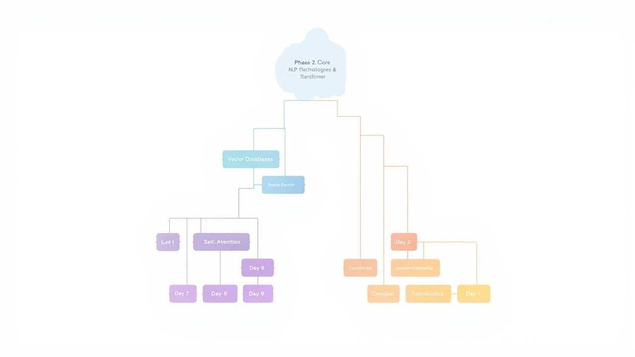
核心概念总结
从 Day 7 到 Day 10:知识图谱
~/ai-agent
关键技术栈
| 技术 |
作用 |
关联 |
| Embedding |
文字 → 向量 |
Day 7 |
| 向量数据库 |
存储/检索向量 |
Day 7 |
| RAG |
检索增强生成 |
Day 7 |
| Self-Attention |
全局依赖建模 |
Day 8 |
| Q, K, V |
注意力三要素 |
Day 8 |
| Multi-Head |
多角度理解 |
Day 8 |
| 位置编码 |
注入位置信息 |
Day 9 |
| Sinusoidal |
固定频率编码 |
Day 9 |
| RoPE |
旋转编码 |
Day 9 |
| Transformer |
完整架构 |
Day 10 |
| Encoder/Decoder |
输入理解/输出生成 |
Day 10 |
| Mask |
防止信息泄露 |
Day 10 |
| Layer Norm |
训练稳定 |
Day 10 |
后续学习路径
~/ai-agent
Phase 2 (Day 7-10) ✅ ──→ Phase 3: RAG & Prompt 工程
                              ├── Day 11: 文档分块策略
                              ├── Day 12: Embeddings 与向量检索
                              └── Day 13: Prompt 工程 (CoT, ReAct)

                                          ↓
                              Phase 4: AI Agent 开发
                              ├── LangChain / LlamaIndex
                              ├── Function Calling
                              └── Dify 低代码平台
参考资源
- 论文: Attention Is All You Need (Vaswani et al., 2017)
- 代码: Day 7-10 各文件夹中的 Demo 代码
- 可视化: 各文件夹中生成的
.png 图片
笔记整理日期:2026-04-11
学习周期:Day 7 - Day 10