当前位置：首页>学习笔记>动手学深度学习 | 笔记07 Softmax回归、损失函数与图片分类数据集

动手学深度学习 | 笔记07 Softmax回归、损失函数与图片分类数据集

2026-04-02 00:11:07

一、Softmax回归

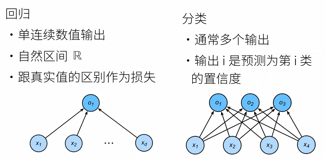
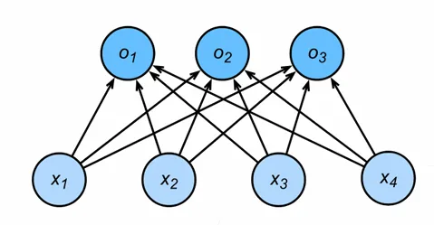
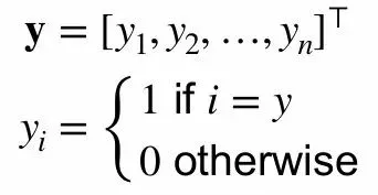
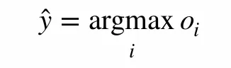
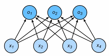
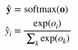
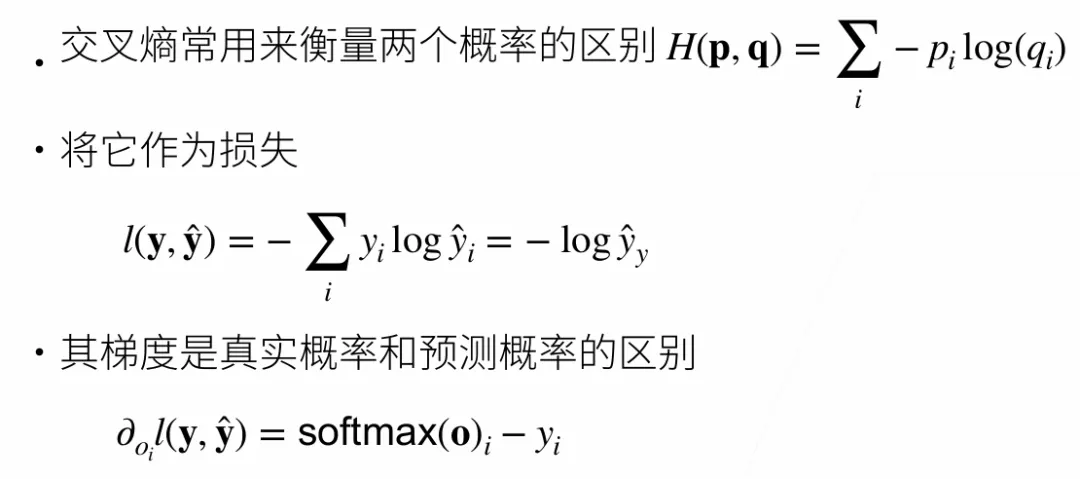
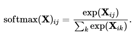
Softmax回归也是机器学习中非常经典且重要的模型。虽然名字叫做回归，但其实是一个分类问题。

回归与分类的区别：

-回归是估计一个连续值

-分类是预测一个离散类别（如MNIST手写数字识别，10类）

从回归过渡到多类分类：均方损失

1.对类别进行一位有效编码（假设真实类别是第i个，那么y_i=1，其他元素均为0）

2.使用均方损失训练

3.最大值作为预测（在作预测的时候，选取i使得最大化o_i的置信度的值作为预测）

这样能确保模型把真正的类和不一样的类拉开距离

4.输出匹配概率（非负，和为1）

5.真实概率y和预测概率y^的区别作为损失

Softmax和交叉熵损失

综上，Softmax回归是一个多类分类模型，使用Softmax操作子可以得到每个类的预测置信度，使用交叉熵来衡量预测和标号的区别作为损失函数

二、损失函数

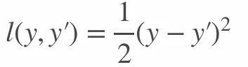
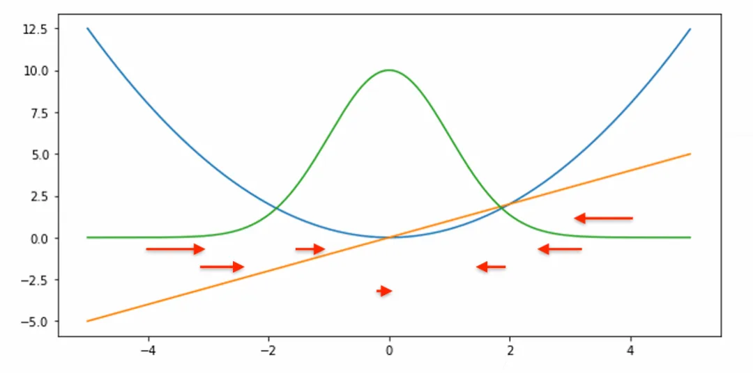
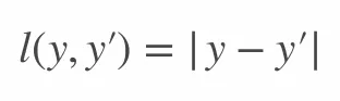
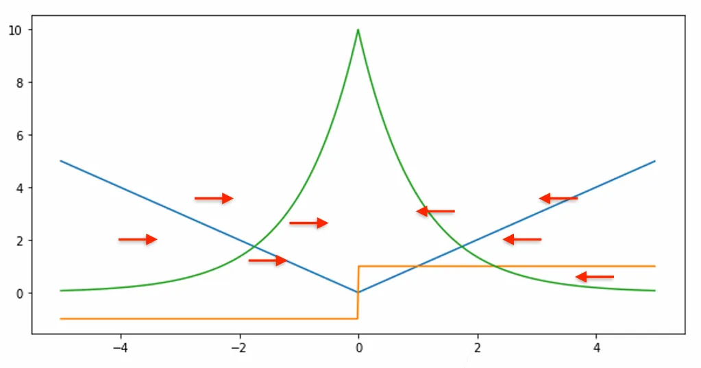
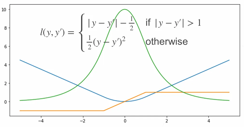
损失函数用来衡量预测值和真实值之间的区别，下面介绍三个常用的损失函数

1.均方损失（L2 Loss）

定义：真实值y - 预测值y'，再做平方，再除以2.

*除以2的意思为方便求导，2与1/2抵消

图像：假设真实值y=0的情况

蓝色曲线：当y=0时，变换预测值y'的函数（二次函数）

绿色曲线：是l的似然函数（e^(-l)），也是高斯分布

橙色直线：损失函数的梯度（过原点的一次函数）

当预测值y'与真实值y隔得比较远的时候，那梯度比较大，所以参数更新比较多

随着真实值慢慢靠近预测值的时候，靠近远点的时候，梯度会变得越来越小，所以参数更新幅度越来越小

但是离原点比较远的时候，不一定想要非常大的梯度来更新参数，所以还有另外一个选择：L1 Loss

不管预测值与真实值隔得有多远，梯度始终为常数，权重更新不会特别大，可以带来稳定性上的好处。

缺点是零点处不可导，不平滑性导致预测值与真实值靠的比较近的时候可能不稳定。

当然，可以提出一个新的函数来结合上面两个函数的好处，并避免劣处，即Huber's Robust Loss

3.Huber's Robust Loss

当预测值和真实值差的比较大的时候，即绝对值大于1时，为绝对值误差；当预测值和真实值比较近的时候，即绝对值小于1时，为均方误差。

这样可以保证优化比较平缓。

三、图像分类数据集

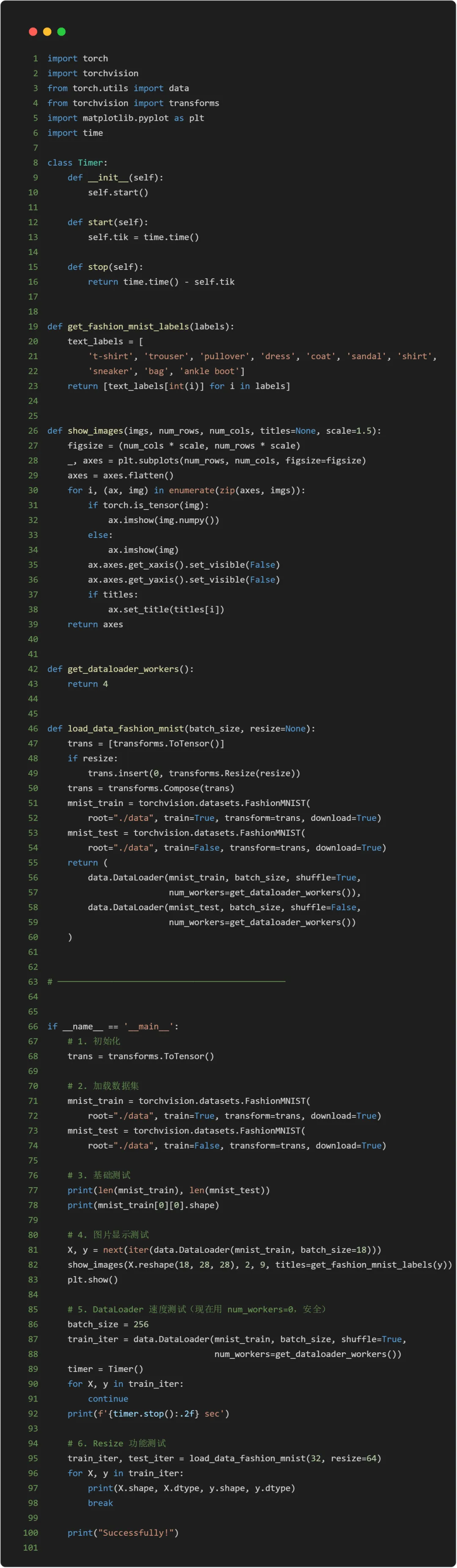
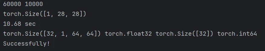
MNIST数据集是图像分类中广泛使用的数据集之一，但作为基准数据集过于简单。所以将使用类似但更复杂的Fashion-MNIST数据集。

import torchimport torchvisionfrom torch.utils import datafrom torchvision import transformsimport matplotlib.pyplot as pltimport time# 通过框架中的内置函数将 Fashion-MNIST 数据集下载并读取到内存中# 通过ToSensor实例将图像数据从PIL类型变换成32位浮点数格式# 并除以255使得所有像素的数值均在0到1之间trans = transforms.ToTensor()mnist_train = torchvision.datasets.FashionMNIST(root="./data", train=True,                                                transform=trans,                                                download=True)mnist_test = torchvision.datasets.FashionMNIST(root="./data", train=False,                                               transform=trans, download=True)print(len(mnist_train), len(mnist_test))#(60000, 10000)

# 第一张图片的形状print(mnist_train[0][0].shape)# torch.Size([1, 28, 28])

# 两个可视化数据集的函数def get_fashion_mnist_labels(labels):      """返回Fashion-MNIST数据集的文本标签。"""    text_labels = [        't-shirt', 'trouser', 'pullover', 'dress', 'coat', 'sandal', 'shirt',        'sneaker', 'bag', 'ankle boot']    return [text_labels[int(i)] for i in labels]def show_images(imgs, num_rows, num_cols, titles=None, scale=1.5):      """Plot a list of images."""    figsize = (num_cols * scale, num_rows * scale)    _, axes = plt.subplots(num_rows, num_cols, figsize=figsize)    axes = axes.flatten()    for i, (ax, img) in enumerate(zip(axes, imgs)):        if torch.is_tensor(img):            ax.imshow(img.numpy())        else:            ax.imshow(img)        ax.axes.get_xaxis().set_visible(False)        ax.axes.get_yaxis().set_visible(False)        if titles:            ax.set_title(titles[i])    return axes

# 几个样本的图像及其相应的标签X, y = next(iter(data.DataLoader(mnist_train, batch_size=18)))show_images(X.reshape(18, 28, 28), 2, 9, titles=get_fashion_mnist_labels(y));# 若是在PyCharm中运行，加上 plt.show()

# 定义Timer()class Timer:    def __init__(self):            self.start()    def start(self):            self.tik = time.time()    def stop(self):            """返回耗时（秒）"""                    return time.time() - self.tik# 读取一小批量数据，大小为batch_size，并输出所需时间batch_size = 256def get_dataloader_workers():    """使用4个进程来读取数据。"""    return 4train_iter = data.DataLoader(mnist_train, batch_size, shuffle=True,                             num_workers=get_dataloader_workers())timer = Timer()for X, y in train_iter:    continuef'{timer.stop():.2f} sec'

以上代码若在本地PyCharm运行，需要稍加修改结构：

输出结果：

综上，我们可以把以上代码结合起来，封装为load_data_fashion_mnist函数

# 定义load_data_fashion_mnist函数def load_data_fashion_mnist(batch_size, resize=None):      """下载Fashion-MNIST数据集，然后将其加载到内存中。"""    trans = [transforms.ToTensor()]    if resize:        trans.insert(0, transforms.Resize(resize))    trans = transforms.Compose(trans)    mnist_train = torchvision.datasets.FashionMNIST(root="./data",                                                    train=True,                                                    transform=trans,                                                    download=True)    mnist_test = torchvision.datasets.FashionMNIST(root="./data",                                                   train=False,                                                   transform=trans,                                                   download=True)    return (data.DataLoader(mnist_train, batch_size, shuffle=True,                            num_workers=get_dataloader_workers()),            data.DataLoader(mnist_test, batch_size, shuffle=False,                            num_workers=get_dataloader_workers()))train_iter, test_iter = load_data_fashion_mnist(32, resize=64)for X, y in train_iter:    print(X.shape, X.dtype, y.shape, y.dtype)    break