有限元基础学习笔记(三)
- 2026-05-23 06:57:26
从公式到代码:1D 有限元 Python 实现
本文我们用 Python 写一个最小 1D 有限元求解 demo,来帮助理解前面推导的公式。
在 FEM 代码里,最机械但关键的工作只有一件事:把弱形式里的积分算出来。
为此需要两块铺垫:等参元 与 高斯积分。
1. 等参元与数值积分
弱形式中最常见的两类积分项(以 1D 杆单元为例)是:
其中, , , 可能随着 变化,积分往往难以解析求出,因此需要数值积分。
1. 高斯积分(Gauss quadrature)
高斯积分 的思想是:把 上的积分用若干采样点的加权求和近似:
其中 是权重,是高斯积分点。
实际问题里,每个单元的积分区间一般是 ,如果直接在 上布置积分点,代码会变得很碎,因为每个单元长度不同,坐标不同,积分点位置也不同。
所以 FEM 通常会先做 等参映射:把所有单元都搬到同一个参考区间 。
2. 等参元(Isoparametric element)
等参元 的思路是:
• 把每个物理单元 都映射到同一个参考单元 。
以二阶三节点单元为例,我们用形函数插值几何坐标:
对 求导:
因此微分关系是:
其中 是 Jacobian(1D为标量)
弱形式里的刚度矩阵需要 ,但形函数天然写在 ,所以要用链式法则把导数换回物理坐标:
3. 任意积分的统一计算
有了等参映射以后,任何 上的积分都能写成:
再用高斯积分得到计算公式:
4.选几个高斯点?
点Gauss–Legendre在上对次数的多项式积分是精确的
实际 FEM 里高斯点个数的选择,取决于你要积分的被积函数最高有多复杂。
经验上可以这样取:
• 刚度矩阵:若 , 在单元内近似常数,线性单元用 1 点即可。 • 体力项:如果 至少是线性的,线性单元通常需要 2 点才能算准。 • 高阶单元一般取 较为合适。
2. 1D 有限元 Python 代码
有限元代码的核心任务是:
计算单元矩阵与向量 → 组装整体方程 → 施加边界条件 → 求解。
本 demo 以之前的 1D 杆问题为例,实现:
• 自定义等分网格 • 自定义单元阶次 • 计算出未知节点位移 • 生成位移场 及应力场
1. 问题描述(problem.py)
仍取前面推文中的案例,具体参数:
• 杆长 , 为常数 • 体力 (或 ) • 左端 :自然边界 • 右端 :本质边界
E = 100000.0
A = 1.0

def q(x):
    return 10.0 * A * x

natural_bcs = {0.0 : 10.0}
essential_bcs = {2.0 : 0.0}
2. 网格(mesh.py)
等分网格要输出两样东西:
• coords: 全局节点坐标• conn: 每个单元包含哪些节点(连通性)
对 阶单元,单元间共享端点,所以总节点数:
import numpy as np
def make_mesh_1d(x0, xl, nel, p):
    """
    x0: float,起点坐标
    x1: float,终点坐标
    nel: int,单元数
    p: int,单元阶数
    """

    nnp = nel * p + 1
    coords = np.linspace(x0, xl, nnp)
    conn = np.zeros((nel, p+1), dtype=int)

    for e in range(nel):
        conn[e, :] = np.arange(e * p, e * p + (p + 1))

    return coords, conn
3. 单元形函数(shape1d.py)
等参坐标 ,等距节点:
Lagrange 形函数:
导数:
def lagrange_shape_1d(p, xi):
    """
    输入:
    p: int,单元阶数
    xi: 等参元坐标,在[-1,1]范围上
    ----------
    输出:
    N: (p+1, ) xi为输入时的形函数值
    dN_dxi: (p+1, ) xi为输入时形函数一阶导数值
    """

    N = np.ones(p+1, dtype=float)
    dN_dxi = np.zeros(p+1, dtype=float)
    xii = np.zeros(p+1, dtype=float)

    ### 对应公式Eq.9
    for i in range(p+1):
        xii[i] = -1 + 2 * i / p
    ### 对应公式Eq.10
    for i in range(p+1):
        for j in range(p+1):
            if i != j:
                N[i] = N[i] * (xi - xii[j]) / (xii[i] - xii[j])
    ### 对应公式Eq.11
    for i in range(p+1):
        term = 0
        for k in range(p+1):
            if k != i:
                prod = 1
                for j in range(p+1):
                    if (j != k) and (j != i):
                        prod = prod * (xi - xii[j]) / (xii[i] - xii[j])
                term += (1/(xii[i] - xii[k])) * prod
        dN_dxi[i] = term

    return N, dN_dxi
4. 数值积分(quad.py)
最小实现:1~3 高斯点,后续可补充。
def gauss_legendre(n_gauss):
    """
    输入:
    n_gauss: int,高斯积分点
    ----------
    输出:
    xi_g: (n_gauss, ) 对应的高斯点坐标
    w_g: (n_gauss, ) 对应的权重
    """
    xi_g = np.zeros(n_gauss)
    w_g = np.zeros(n_gauss)

    if n_gauss == 1:
        w_g[0] = 2.0
        xi_g[0] = 0.0
    elif n_gauss == 2:
        xi_g[:] = [-0.5773502691896257, 0.5773502691896257]
        w_g[:]  = [1.0, 1.0]
    elif n_gauss == 3:
        xi_g[:] = [-0.7745966692414834, 0.0, 0.7745966692414834]
        w_g[:]  = [0.5555555555555556, 0.8888888888888888, 0.5555555555555556]
    else:
        raise ValueError("n must be 1, 2, or 3 in this demo.")

    return xi_g, w_g
5. 单元矩阵与向量(element1d.py)
单元积分统一写成参考单元 上的求和:
每个高斯点的计算顺序很固定:
Step 1 形函数与导数:
Step 2 物理坐标:
Step 3 Jacobian:
Step 4 矩阵:
Step 5 累加 :
Step 6 累加 :
import numpy as np
from quad import *
from shape1d import *
from problem import *

def element_matrices(coords_e, p, n_gauss):
    """
    输入:
    coords_e: 单元物理坐标
    p: 单元阶次
    n_gauss: 高斯点个数
    ----------
    输出:
    Ke: (p+1, p+1) 单元刚度矩阵
    fe: (p+1, ) 单元外荷载向量
    """
    nen = p+1           # 单元节点数
    Ke = np.zeros((nen, nen))
    fe = np.zeros(nen)

    xi_g, w_g = gauss_legendre(n_gauss)

    for i in range(n_gauss):
        xi = xi_g[i]
        w = w_g[i]
        # Step 1: N, dN/dxi
        N, dN_dxi = lagrange_shape_1d(p, xi)
        # Step 2: x(xi)
        x = N @ coords_e
        # Step 3: J(xi)
        J = dN_dxi @ coords_e
        # Step 4: B = dN/dx
        dN_dx = dN_dxi / J
        B = dN_dx
        # Step 5: Ke
        Ke += (E*A) * np.outer(B, B) * (w * J)
        # Step 6: fe (body force)
        fe += N * q(x) * (w * J)

    return Ke, fe
6. 组装与求解(solver1d.py)
组装整体矩阵
前面刚好有一个变量 conn 定义是的各单元内节点的编号。
import numpy as np
from mesh import *
from element1d import *
from problem import *

def assemble_global(coords, conn, p, n_gauss):
    """
    输入:
    coords: 所有节点物理坐标
    conn: 各单元上的节点ID
    p: 单元阶次
    n_gauss: 高斯点个数
    ----------
    输出:
    K: (ndofs, ndofs) 整体刚度矩阵
    f: (ndofs, ) 整体外荷载向量
    """
    ndofs = coords.shape[0]  # 总自由度
    nele = conn.shape[0]   # 总单元数

    K = np.zeros((ndofs, ndofs))
    F = np.zeros(ndofs)

    for e in range(nele):
        edofs = conn[e, :]  # 各单元内自由度编号,如[0, 1, 2]
        coords_e = coords[edofs]

        ke, fe = element_matrices(coords_e, p, n_gauss)

        for i in range(p+1):
            F[edofs[i]] += fe[i]   #单元e中第i个自由度在整体中的编号edofs[i]
            for j in range(p+1):
                K[edofs[i], edofs[j]] += ke[i, j]
    return K, F
施加边界条件并求解
这里做两件事:
• 自然边界 加到载荷向量 F 上 • 本质边界 通过分块消元求解未知自由度
本 demo 只处理每类 BC 各 1 个的情况。
对 按照自由度进行分块得:
通过第二行公式来求解未知位移:
def apply_bcs_and_solve(K, F, coords):
    """
    输入:
    K: (ndofs, ndofs) 整体刚度矩阵
    F: (ndofs, ) 整体外荷载向量
    coords: (ndofs, ) 所有节点坐标
    ----------
    输出:
    d: (ndofs, ) 整体节点位移
    """

    ndofs = K.shape[0]
    # 施加自然边界条件(牵引力)
    x_t = list(natural_bcs.keys())[0]
    tbar = natural_bcs[x_t] * A
    node_t = np.where(np.isclose(coords, x_t))[0][0]    #vaule
    F[node_t] += tbar

    # 施加本质边界条件(位移)
    x_u = list(essential_bcs.keys())[0]    # list
    ubar = essential_bcs[x_u]

    fixed = np.where(np.isclose(coords, x_u))[0] #分块,本质边界条件节点id的list
    fixed_set = set(fixed.tolist())
    free = np.array([i for i in range(ndofs) if i not in fixed_set], dtype=int)  # 分块,其他节点id的list

    # 分块矩阵
    K_FF = K[free][:, free]
    K_FE = K[free][:, fixed]
    F_F = F[free]

    # 施加本质边界条件(位移)
    d_E = np.array([ubar], dtype=float)

    # 求解得未知节点位移
    rhs = F_F - K_FE @ d_E
    d_F = np.linalg.solve(K_FF, rhs)

    d = np.zeros(ndofs)
    d[fixed] = d_E
    d[free] = d_F

    return d
后处理
在每个单元 上取若干采样点 ,计算:
Step 1:
Step 2:
Step 3:
Step 4:
def evaluate_uh_on_mesh(coords, conn, p, d, nplot_per_elem=50):
    """
    输入:
    coords: 所有节点物理坐标
    conn: 各单元上的节点ID
    p: 单元阶次
    d: 所有节点位移
    nplot_per_elem: 每个单元上采样点
    ----------
    输出:
    x_h, u_h, eps_h, sigma_h: 全场结果
    """

    nel = conn.shape[0]
    xi_grid = np.linspace(-1.0, 1.0, nplot_per_elem)

    X_all, U_all, EPS_all, SIG_all = [], [], [], []

    for e in range(nel):
        # 每个单元上的节点id
        enodes = conn[e, :]
        coords_e = coords[enodes]              # (p+1,)
        de = d[enodes]                   # (p+1,)

        xi_use = xi_grid

        for xi in xi_use:
            # 形函数及一阶导数
            N, dN_dxi = lagrange_shape_1d(p, xi)

            # 等参变换 Step 1
            x = N @ coords_e  # 每个单元采样点对应的物理坐标
            J = dN_dxi @ coords_e

            # 位移 Step 2
            u = N @ de

            X_all.append(x)
            U_all.append(u)


            # dN/dx = (dN/dxi)/J
            dN_dx = dN_dxi / J
            # 应变和应力 Step 3 and 4
            eps = dN_dx @ de
            sig = E * eps

            EPS_all.append(eps)
            SIG_all.append(sig)

    x_h =  np.array(X_all, dtype=float)
    u_h =  np.array(U_all, dtype=float)
    eps_h = np.array(EPS_all, dtype=float)
    sigma_h = np.array(SIG_all, dtype=float)

    return x_h, u_h, eps_h, sigma_h
3. 案例计算
有以上代码后,我们可以在main.py里创建一个函数用于计算。
import numpy as np
from problem import *
from mesh import *
from shape1d import *
from quad import *
from element1d import *
from solver1d import *

def run_case(x0, x1, nel, p, n_gauss, nplot_per_elem=50):

    coords, conn = make_mesh_1d(x0, x1, nel, p)

    K, F = assemble_global(coords, conn, p, n_gauss)
    d = apply_bcs_and_solve(K, F, coords)

    x_plot, u_h, eps_h, sigma_h = evaluate_uh_on_mesh(
        coords, conn, p, d, nplot_per_elem=nplot_per_elem
    )

return x_plot, u_h, sigma_h然后可以自定义nel, p, n_gauss这三个参数。我们先固定单元数,比较不同的p 和 n_gauss:
1. nel=2,p=1,n_gauss=12. nel=2,p=1,n_gauss=23. nel=2,p=2,n_gauss=24. nel=2,p=3,n_gauss=3
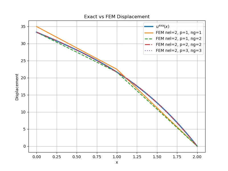
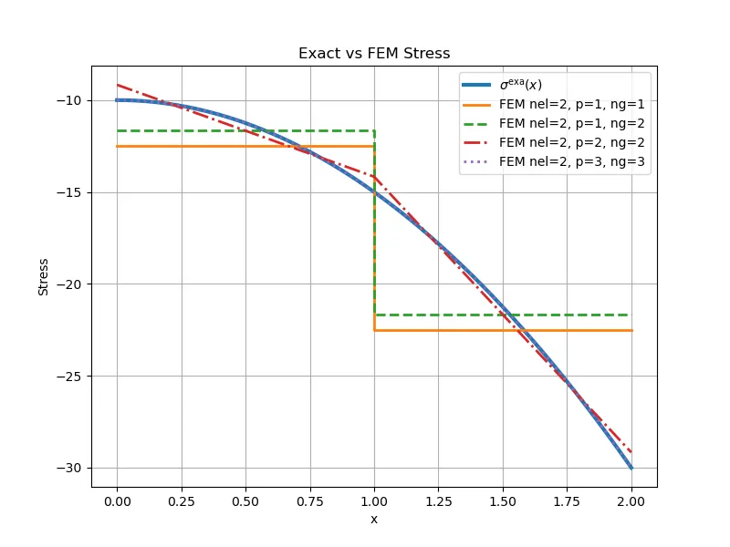
可以看出:
• 1 与 2 的位移不重合,其主要原因来自体力项积分:本例中 是线性的,线性单元 是一次,因此被积函数最高为二次,1 点Gauss 不能精确积分二次项。改用 2 点后明显改善。 • 3 与 4(高阶单元)位移更接近精确解:高阶单元在单元内允许更高次数的位移多项式,自然更容易拟合精确位移曲线。 • 应力只有 4 更贴近精确解:三次单元位移是三次多项式,因此应变/应力是二次多项式,能更好逼近本例精确应力。
进一步,固定单元阶数和高斯积分点,我们变化单元数:
5. nel=5 ,p=1, n_gauss=1
6. nel=10 ,p=1, n_gauss=1
以下为计算结果:
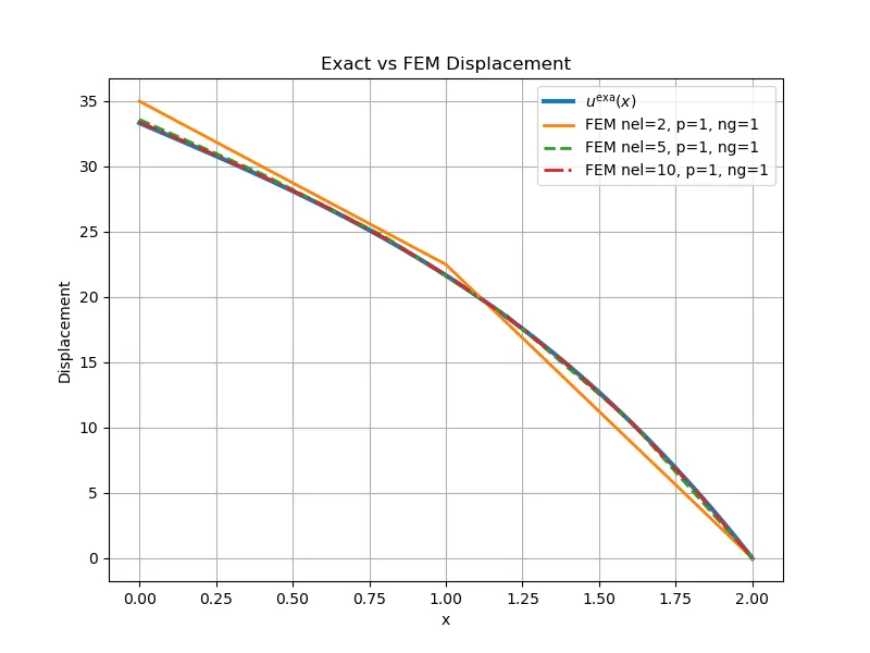
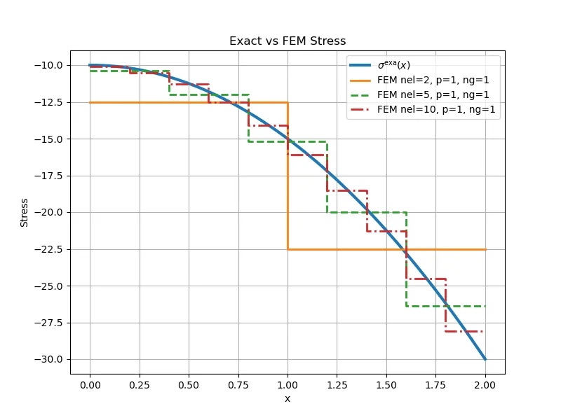
可以看出:
• 当我们增加单元数时,位移会逐步收敛到精确解。 • 但 在每个线性单元内恒为常数,所以应力曲线必然是“阶梯状”。加密网格只能让阶梯更细,并不会让它真正变光滑。想得到更光滑、更准确的应力分布,通常需要用高阶单元或应力恢复。

