PyTorch学习笔记|单层神经网络
- 2026-05-15 20:49:37

单层回归网络
其实神经网络并不复杂,我们经过前面的铺垫,如果只看单层的网络(输入层不算),其实就是下面这张图片,好像其实也就是一个线性回归的方程,当然神经网络只所以好用,是因为有多层网络和非线性的激活函数,这个我们后面再来说。
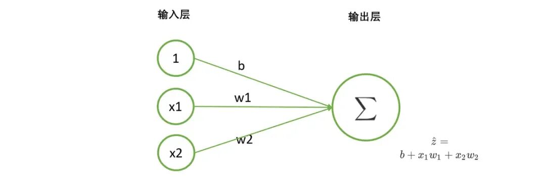
那我们先用tensor来实现一下神经网络的正向传播。
import torch

X = torch.tensor([[1,0,0],[1,1,0],[1,0,1],[1,1,1]], dtype = torch.float32)
w = torch.tensor([-0.2, 0.15, 0.15])
z = torch.tensor([-0.2, -0.05, -0.05, 0.1])

def Linear(X, w):
    zhat = torch.mv(X, w)
    return zhat

zhat = Linear(X,w)
print(zhat)

#tensor([-0.2000, -0.0500, -0.0500,  0.1000])
nn.Linear实现单层回归网络
当然,我们在pytorch中有专门的类用来创建单层回归网络,我们来看一下代码。
X = torch.tensor([[0,0],[1,0],[0,1],[1,1]], dtype = torch.float32)
output = torch.nn.Linear(2,1)
zhat = output(X)
print(zhat)

#result
tensor([[ 0.4556],
        [-0.2170],
        [ 1.0687],
        [ 0.3961]], grad_fn=<AddmmBackward0>)
通过上面代码,我们需要注意几个点: 一是我们看下LInear中的2和1是什么含义,2是in_features,也就是输入数据的特征数量(两个特征,也就是X数据的2列),1是out_features,也就是输出是一个神经元。 二是有没有发现输入的X和我们之前写的少了全是1的一列,因为LInear会自动帮我们生成b偏置数据。 三是我们没有定义w和b,这些是自动生成的随机数,我们可以打印出来看看。
X = torch.tensor([[0,0],[1,0],[0,1],[1,1]], dtype = torch.float32)
output = torch.nn.Linear(2,1)
zhat = output(X)
print(output.weight, output.bias)
print(output.weight.shape, output.bias.shape)
print(zhat.shape)

# result
Parameter containing:
tensor([[0.1488, 0.0206]], requires_grad=True) Parameter containing:
tensor([0.4631], requires_grad=True)
torch.Size([1, 2]) torch.Size([1])
torch.Size([4, 1])
当然我们也可以不要偏置。
output = torch.nn.Linear(2,1,bias=False)
进一步讨论nn.Linear
看完上面的内容,我还是想要了解w和b生成后是怎么计算的,为什么我会有这样的疑问了,因为各种教程在讲解这部分内容写矩阵表达式的时候各不同,用wX,有wTX,还有返回来的Xw和XwT,当然这些都对,只要我们设置好数据的形状格式,那我就想知道pytorch到底是怎么计算的,那我们就来研究下。
我们还是先看上面案例的返回结果,w的形状是(1,2),其实是(out_features,in_features),我们的X形状是(4,2),所以我初步想的是X*wT。然后bias是[1],所以是在加上bias,然后利用广播运算,这样就能得到最后结果。
# result
Parameter containing:
tensor([[0.1488, 0.0206]], requires_grad=True) Parameter containing:
tensor([0.4631], requires_grad=True)
torch.Size([1, 2]) torch.Size([1])
torch.Size([4, 1]
我们进一步看看源码来验证一下我的想法,确实是这样的。
       self.in_features = in_features
        self.out_features = out_features
        self.weight = Parameter(
            torch.empty((out_features, in_features), **factory_kwargs)
        )
        if bias:
            self.bias = Parameter(torch.empty(out_features, **factory_kwargs))
        else:
            self.register_parameter("bias", None)
        self.reset_parameters()


def linear(input: Tensor, weight: Tensor, bias: Optional[Tensor] = None) -> Tensor:
    # input:  [batch, in_features]
    # weight: [out_features, in_features]
    # bias:   [out_features]

    自动对 weight 做转置 .T,然后矩阵乘法
    output = input @ weight.T

    if bias is not None:
        output += bias #广播运算
    return output
我们把输出改成三个神经元,我们再来加深一下印象。
X = torch.tensor([[0,0],[1,0],[0,1],[1,1]], dtype = torch.float32)
output = torch.nn.Linear(2,3)
zhat = output(X)
print(zhat)
print(zhat.shape)
print(output.weight, output.bias)
print(output.weight.shape, output.bias.shape)

# result
tensor([[-0.6868,  0.7037,  0.2460],
        [ 0.0118,  1.1411,  0.8687],
        [-0.1429,  0.2609,  0.0204],
        [ 0.5557,  0.6983,  0.6431]], grad_fn=<AddmmBackward0>)
torch.Size([4, 3])
Parameter containing:
tensor([[ 0.6986,  0.5439],
        [ 0.4374, -0.4428],
        [ 0.6227, -0.2256]], requires_grad=True) Parameter containing:
tensor([-0.6868,  0.7037,  0.2460], requires_grad=True)
torch.Size([3, 2]) torch.Size([3])
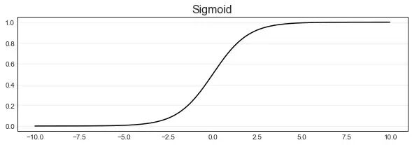
二分类:逻辑回归
当然,现实中我们除了要做回归外,还要做一些分类任务,那就有一个大名鼎鼎的函数sigmoid,这样规定大于0.5时,预测结果为1类, 小于0.5时,预测结果为0类,则可以顺利将回归算法转化为分类算法。
X = torch.tensor([[0,0],[1,0],[0,1],[1,1]], dtype = torch.float32)
output = torch.nn.Linear(2,1)
zhat = output(X)
sigma = torch.sigmoid(zhat)
result  = torch.where(sigma >= 0.5, torch.tensor(1.0), torch.tensor(0.0))
print(sigma)
print(result)

#result
tensor([[0.6020],
        [0.4350],
        [0.5257],
        [0.3607]], grad_fn=<SigmoidBackward0>)
tensor([[1.],
        [0.],
        [1.],
        [0.]])
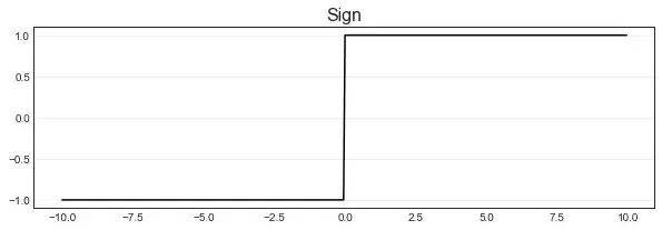
还有其他的函数,我们也来一一介绍一下。
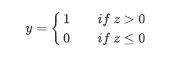
阶跃函数sign
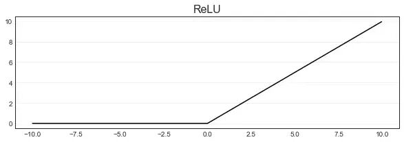
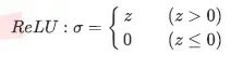
ReLU函数
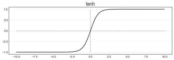
tanh函数
。
torch.sign(zhat)
torch.relu(zhat)
torch.tanh(zhat)
需要注意的是,还可以用nn中的functional来调用,有的会报提醒,说是方法弃用了。
import torch
import torch.nn.functional as F

X = torch.tensor([[0,0],[1,0],[0,1],[1,1]], dtype = torch.float32)
output = torch.nn.Linear(2,1)
zhat = output(X)
print(F.sigmoid(zhat))
多分类:Softmax回归
对于多分类来说,我们就要用到Softmax回归。
需要注意的是,由于softmax的分子和分母中都带有为底的指数函数,所以在计算中非常容易出现极大的数值,用torch来计算就不会出现这样的问题,帮我们处理好了。
X = torch.tensor([[0,0],[1,0],[0,1],[1,1]], dtype = torch.float32)
output = torch.nn.Linear(2,3)
zhat = output(X)
sigma = torch.softmax(zhat,dim=1) #一定要加dim参数,此时需要进行加和的维度是1
print(sigma.shape,sigma)

#result
torch.Size([4, 3]) tensor([[0.3028, 0.2799, 0.4173],
        [0.2970, 0.1531, 0.5500],
        [0.3278, 0.2946, 0.3776],
        [0.3279, 0.1644, 0.5077]], grad_fn=<SoftmaxBackward0>)

